Python pandas (Grouping)
Table of Contents
Overview
In the previous discussion on py pandas, we explored the capabilities of Python Pandas for data analysis and manipulation. In this continuation, I will delve deeper into practical applications, specifically addressing methodologies for extracting and analyzing data within this framework.
Data
Again we need som data, but this time lets start with something really simple. Something that makes it easier to understand and comprehend. Lets consider a bike race tour. The tour data:
| Name | Stage | Gender | Time | Egap | Watts |
|---|---|---|---|---|---|
| Calle | 1 | M | 1:21:00.123 | 0:30.045 | 285 |
| Calle | 2 | M | 0:59:12.234 | 0:25.234 | 320 |
| Calle | 3 | M | 1:10:00.434 | 0:05.234 | 300 |
| Alice | 1 | F | 1:10:15.543 | 0:55.000 | 250 |
| Alice | 2 | F | 0:54:20.987 | 0:45.456 | 230 |
| Bob | 1 | M | 0:45:05.789 | 0:01.234 | 335 |
| Oscar | 2 | M | 1:05:30.456 | 0:15.789 | 310 |
| Oscar | 3 | M | 0:59:45.123 | 0:00.000 | 340 |
| Eve | 1 | F | 0:50:30.103 | 0:20.000 | 220 |
| Frank | 2 | M | 0:58:10.234 | 0:10.000 | 260 |
| Grace | 1 | F | 0:40:20.987 | 0:38.456 | 275 |
| Grace | 2 | F | 1:15:15.654 | 0:55.789 | 300 |
| Grace | 3 | F | 1:00:00.321 | 0:01.000 | 290 |
| Hank | 3 | M | 0:45:15.456 | 0:40.000 | 230 |
| Isla | 1 | F | 1:05:05.001 | 0:30.500 | 345 |
| Jack | 2 | M | 0:50:25.678 | 0:00.123 | 255 |
| Jack | 3 | M | 1:12:10.000 | 0:03.000 | 275 |
Lets make our first DataFrame, for this we use the header of the table as column names. Lets checkout that we have what we want:
import pandas as pd

org_df =pd.DataFrame(columns=header,data=data)
print(org_df)
     Name  Stage Gender         Time      Egap  Watts
0   Calle      1      M  1:21:00.123  0:30.045    285
1   Calle      2      M  0:59:12.234  0:25.234    320
2   Calle      3      M  1:10:00.434  0:05.234    300
3   Alice      1      F  1:10:15.543  0:55.000    250
4   Alice      2      F  0:54:20.987  0:45.456    230
5     Bob      1      M  0:45:05.789  0:01.234    335
6   Oscar      2      M  1:05:30.456  0:15.789    310
7   Oscar      3      M  0:59:45.123  0:00.000    340
8     Eve      1      F  0:50:30.103  0:20.000    220
9   Frank      2      M  0:58:10.234  0:10.000    260
10  Grace      1      F  0:40:20.987  0:38.456    275
11  Grace      2      F  1:15:15.654  0:55.789    300
12  Grace      3      F  1:00:00.321  0:01.000    290
13   Hank      3      M  0:45:15.456  0:40.000    230
14   Isla      1      F  1:05:05.001  0:30.500    345
15   Jack      2      M  0:50:25.678  0:00.123    255
16   Jack      3      M  1:12:10.000  0:03.000    275
Grouping basically means that we want to group certain fields, for example we might want to group by stage or by name. This means that we create groups with each individual name (or stage).
Lets give it a try:
riders = org_df.groupby('Name')
print(riders.groups)
print("----------")
stages = org_df.groupby('Stage')
print(stages.groups)
{'Alice': [3, 4], 'Bob': [5], 'Calle': [0, 1, 2], 'Eve': [8], 'Frank': [9], 'Grace': [10, 11, 12], 'Hank': [13], 'Isla': [14], 'Jack': [15, 16], 'Oscar': [6, 7]}
----------
{1: [0, 3, 5, 8, 10, 14], 2: [1, 4, 6, 9, 11, 15], 3: [2, 7, 12, 13, 16]}
In the above exampe we can see , that each group starts with the name, or a stage that means that we can retrieve a specific group and examine that some more. In the below code, Jack-group is retrieved, and then outputs the watts. We also take a look at stage 2, which Names were paricpating, and what were the individual times for that stage?
print(riders.get_group('Jack')['Watts'])
print(f"Stage 2\n{stages.get_group(2)[['Name','Time']]}")
15    255
16    275
Name: Watts, dtype: int64
Stage 2
     Name         Time
1   Calle  0:59:12.234
4   Alice  0:54:20.987
6   Oscar  1:05:30.456
9   Frank  0:58:10.234
11  Grace  1:15:15.654
15   Jack  0:50:25.678
We could also iterate through the groups. As in the code below, this
will return two fields: The first is the grouping field (Name). The
other is the DataFrame values (Index, Name, Stage, Gender, Egap, Watts).
If we wanted we could pick out the values that we are intrested in for
example ['Watts']
for name, grp in riders:
    print(f"name: {name} vals: {grp}")
name: Alice vals:     Name  Stage Gender         Time      Egap  Watts
3  Alice      1      F  1:10:15.543  0:55.000    250
4  Alice      2      F  0:54:20.987  0:45.456    230
name: Bob vals:   Name  Stage Gender         Time      Egap  Watts
5  Bob      1      M  0:45:05.789  0:01.234    335
name: Calle vals:     Name  Stage Gender         Time      Egap  Watts
0  Calle      1      M  1:21:00.123  0:30.045    285
1  Calle      2      M  0:59:12.234  0:25.234    320
2  Calle      3      M  1:10:00.434  0:05.234    300
name: Eve vals:   Name  Stage Gender         Time      Egap  Watts
8  Eve      1      F  0:50:30.103  0:20.000    220
name: Frank vals:     Name  Stage Gender         Time      Egap  Watts
9  Frank      2      M  0:58:10.234  0:10.000    260
name: Grace vals:      Name  Stage Gender         Time      Egap  Watts
10  Grace      1      F  0:40:20.987  0:38.456    275
11  Grace      2      F  1:15:15.654  0:55.789    300
12  Grace      3      F  1:00:00.321  0:01.000    290
name: Hank vals:     Name  Stage Gender         Time      Egap  Watts
13  Hank      3      M  0:45:15.456  0:40.000    230
name: Isla vals:     Name  Stage Gender         Time      Egap  Watts
14  Isla      1      F  1:05:05.001  0:30.500    345
name: Jack vals:     Name  Stage Gender         Time      Egap  Watts
15  Jack      2      M  0:50:25.678  0:00.123    255
16  Jack      3      M  1:12:10.000  0:03.000    275
name: Oscar vals:     Name  Stage Gender         Time      Egap  Watts
6  Oscar      2      M  1:05:30.456  0:15.789    310
7  Oscar      3      M  0:59:45.123  0:00.000    340
So we manage to get groups based on a column, but maybe we want more. In this case we want to group both Name and Stage and pick out the Time.
multi_gr= org_df.groupby(['Name','Stage'])

for (name,stage),val in multi_gr:
    print(f"name: {name} stage:{stage}  Time: {val['Time'].to_numpy()[0]}")
name: Alice stage:1  Time: 1:10:15.543
name: Alice stage:2  Time: 0:54:20.987
name: Bob stage:1  Time: 0:45:05.789
name: Calle stage:1  Time: 1:21:00.123
name: Calle stage:2  Time: 0:59:12.234
name: Calle stage:3  Time: 1:10:00.434
name: Eve stage:1  Time: 0:50:30.103
name: Frank stage:2  Time: 0:58:10.234
name: Grace stage:1  Time: 0:40:20.987
name: Grace stage:2  Time: 1:15:15.654
name: Grace stage:3  Time: 1:00:00.321
name: Hank stage:3  Time: 0:45:15.456
name: Isla stage:1  Time: 1:05:05.001
name: Jack stage:2  Time: 0:50:25.678
name: Jack stage:3  Time: 1:12:10.000
name: Oscar stage:2  Time: 1:05:30.456
name: Oscar stage:3  Time: 0:59:45.123
We can conclude that if we have a multi groupby and iterate over the groups, the first is a tuple in which the groupby criteria is available.
So lets go back for a second.. Lets get all the fields for rider Calle.
calle_rider = org_df[org_df['Name'] == 'Calle']


print(calle_rider)
    Name  Stage Gender         Time      Egap  Watts
0  Calle      1      M  1:21:00.123  0:30.045    285
1  Calle      2      M  0:59:12.234  0:25.234    320
2  Calle      3      M  1:10:00.434  0:05.234    300
Could we use that to group by stage? The code below will group only the values from calle, into groups separated by stage, and get the Time value for each stage.
calle_groups = calle_rider.groupby('Stage')

for stage, vals in calle_groups:
    print(f"stage: {stage} vals: {vals['Time']}")
stage: 1 vals: 0    1:21:00.123
Name: Time, dtype: object
stage: 2 vals: 1    0:59:12.234
Name: Time, dtype: object
stage: 3 vals: 2    1:10:00.434
Name: Time, dtype: object
Now, maybe we want to filter out all the groups that did not participate in all three stages.
- Get groups based on names
- Filter out all groups with nth (0,1,2) row, in our case we have 3 rows for each group that has particpated in all three stages.
name_group = org_df.groupby('Name')[['Name','Stage']]
print(name_group.nth(2))
     Name  Stage
2   Calle      3
12  Grace      3
The nth takes the row from each group. In this case the only one who participated in all three stages would have nth(2) (0,1,2). That was kind of cheating, so lets do it with a UDF (User defined filter). First we create a new group with the riders name. Then we filter out all rider that has more than 2 stages in their group.
all_stages = org_df.groupby('Name')
riders_all_stages=all_stages.filter(lambda x: x['Stage'].count() > 2)
print(riders_all_stages[['Name', 'Stage', 'Time']])
     Name  Stage         Time
0   Calle      1  1:21:00.123
1   Calle      2  0:59:12.234
2   Calle      3  1:10:00.434
10  Grace      1  0:40:20.987
11  Grace      2  1:15:15.654
12  Grace      3  1:00:00.321
We want to see the total time for these two gladiators that manage to participate in all three stages.
1:
2: print(f"Sum of riders: {riders_all_stages['Time'].sum()}") #
3: df_copy = org_df.copy()
4:
5: df_copy['Time'] = pd.to_timedelta(df_copy['Time'] )
6: riders_cp = df_copy.groupby('Name')
7: rider_all_stages=riders_cp.filter(lambda x: x['Stage'].count() > 2)
8:
9: print(rider_all_stages)
Sum of riders: 1:21:00.1230:59:12.2341:10:00.4340:40:20.9871:15:15.6541:00:00.321
     Name  Stage Gender                   Time      Egap  Watts
0   Calle      1      M 0 days 01:21:00.123000  0:30.045    285
1   Calle      2      M 0 days 00:59:12.234000  0:25.234    320
2   Calle      3      M 0 days 01:10:00.434000  0:05.234    300
10  Grace      1      F 0 days 00:40:20.987000  0:38.456    275
11  Grace      2      F 0 days 01:15:15.654000  0:55.789    300
12  Grace      3      F 0 days 01:00:00.321000  0:01.000    290
Line 1 concatenated the time since the time was consider a string, this is definitely not what we wanted. Somehow we need to convert the Time string to a timedelta, fortunately we can use the pandas.to_timedelta function to convert all the time to a timedelta object and then write it into the Time column. We could also make it a new field, but in this case we just overwrite the old Time. Now back to our original question how can we get the sum of each rider?
print(rider_all_stages.groupby('Name')['Time'].sum())
print(rider_all_stages.groupby('Name')['Time'].describe())
Name
Calle   0 days 03:30:12.791000
Grace   0 days 02:55:36.962000
Name: Time, dtype: timedelta64[ns]
      count                       mean  ...                     75%                     max
Name                                    ...
Calle     3  0 days 01:10:04.263666666  ...  0 days 01:15:30.278500  0 days 01:21:00.123000
Grace     3  0 days 00:58:32.320666666  ...  0 days 01:07:37.987500  0 days 01:15:15.654000

[2 rows x 8 columns]
Here is a solution: First we group the Name this will create groups for each rider, then we get the Time column (which is now a deltatime) and apply the sum to all the values. Voliá! Another cool feature is the describe, which will generate a descriptive statistics, this too is a DataFrame which means that you could do something like:
all_rider_descr = rider_all_stages.groupby('Name')['Time']

print(f"Calle:\n{all_rider_descr.get_group('Calle').describe()}")
Calle:
count                            3
mean     0 days 01:10:04.263666666
std      0 days 00:10:53.952910262
min         0 days 00:59:12.234000
25%         0 days 01:04:36.334000
50%         0 days 01:10:00.434000
75%         0 days 01:15:30.278500
max         0 days 01:21:00.123000
Name: Time, dtype: object
Maybe we want some more info, for example for each rider we want to see the total amount of time, and the some statistics about the watts over the entire tour.
test_1 = rider_all_stages.groupby('Name')
for name,riders in test_1:
    print(f"name: {name} {riders['Time'].sum()} \n----Watts----\n{riders['Watts'].describe()}")
name: Calle 0 days 03:30:12.791000
----Watts----
count      3.000000
mean     301.666667
std       17.559423
min      285.000000
25%      292.500000
50%      300.000000
75%      310.000000
max      320.000000
Name: Watts, dtype: float64
name: Grace 0 days 02:55:36.962000
----Watts----
count      3.000000
mean     288.333333
std       12.583057
min      275.000000
25%      282.500000
50%      290.000000
75%      295.000000
max      300.000000
Name: Watts, dtype: float64
Plotting
Lets make some visuals. We already seen how we can extract data and how to manipluate data, but nothing is more fun than visualizing the data.
So lets do that. Lets start from scratch, we create our DataFrame provided from the same table.
import pandas as pd
import matplotlib.pyplot as plt
import matplotlib

indexs = [ name[0] for name in data]
df=pd.DataFrame(data=data, columns=header)
#df.set_index('Name',inplace=True)
print(df)
     Name  Stage Gender         Time      Egap  Watts
0   Calle      1      M  1:21:00.123  0:30.045    285
1   Calle      2      M  0:59:12.234  0:25.234    320
2   Calle      3      M  1:10:00.434  0:05.234    300
3   Alice      1      F  1:10:15.543  0:55.000    250
4   Alice      2      F  0:54:20.987  0:45.456    230
5     Bob      1      M  0:45:05.789  0:01.234    335
6   Oscar      2      M  1:05:30.456  0:15.789    310
7   Oscar      3      M  0:59:45.123  0:00.000    340
8     Eve      1      F  0:50:30.103  0:20.000    220
9   Frank      2      M  0:58:10.234  0:10.000    260
10  Grace      1      F  0:40:20.987  0:38.456    275
11  Grace      2      F  1:15:15.654  0:55.789    300
12  Grace      3      F  1:00:00.321  0:01.000    290
13   Hank      3      M  0:45:15.456  0:40.000    230
14   Isla      1      F  1:05:05.001  0:30.500    345
15   Jack      2      M  0:50:25.678  0:00.123    255
16   Jack      3      M  1:12:10.000  0:03.000    275
DateTime in matplotlib
Before we are making plots, we need to be able to handle date and times correctly This has proven to be more trickier than one expects. So lets dig into it, to make it easier to understand lets create a table
| Name | Time |
|---|---|
| Calle | 01:21:00.123 |
| Alice | 01:18:22.566 |
| Sven | 00:59:00.100 |
This should be a simple example showing bar plot on the three different times
import matplotlib as mpl
import matplotlib.pyplot as plt
import matplotlib.dates as mdates
import matplotlib.ticker as tick
from datetime import time,datetime
import pandas as pd


def convert_to_datetime(time_str):
  # Dummy implementation, update according to your needs
   return time.fromisoformat(time_str)


df=pd.DataFrame(data=data, columns=header)
#df['dtobj'] = df['Time'].apply(convert_to_datetime)
df['TimeDelta'] = pd.to_timedelta(df['Time'])


fig,ax = plt.subplots()
ax.bar(df['Name'], df['TimeDelta'].dt.total_seconds())
ax.set_yticks(df['TimeDelta'].dt.total_seconds())


ax.set_yticklabels(df['TimeDelta'].apply(lambda x:
            f'{int(x.components.hours):02}:{int(x.components.minutes):02}:'
            f'{int(x.components.seconds):02}.{int(x.microseconds/1000):03}'))

plt.xlabel('Name')
plt.ylabel('Time (H:M:S.msec)')

plt.tight_layout()
#plt.show()

# Save the plot to a file
output_file = 'bar_plot_times.png'
plt.savefig(output_file)

# Create a link to the output file
print(f'[[file:{output_file}]]')
Lets consider the code above and lets dig into some of the parts
Converting times
Currently we are stuck with the format 01:21:00.123 for example, to make it more abstract we could say its hh:mm:ss.fff. Fortunatly for this string is easily convertible to a datetime.deltatime object which then can be used to do all kinds of manipulations.
But lets consider a different time format, In this case the the string cannot be transformed using deltatimes, since its a non-standard format.
| Name | Time |
|---|---|
| Adam | 1#22.23,1 |
| Beatrice | 0#34.23,4 |
Its necessary to transform the time-str to a deltatime , this can be done in many different ways. If the time is of a stadard format its possible to use pandas.to_timedelta as in line 16. But as in the case above that is not possible. On the other hand , its possible to use something more abstract as for example apply, which will call a function for each of the items in the field and when parsed we construct the timedelta object as in line 9
 1: import pandas as pd
 2: from datetime import timedelta
 3:
 4: def parse_time(time_str:str)->timedelta:
 5:     hours, rest =time_str.split("#")
 6:     minutes, rest = rest.split('.')
 7:     seconds, milliseconds = rest.split(',')
 8:     tmd = timedelta(hours=int(hours), minutes=int(minutes),
 9:               seconds=int(seconds), milliseconds=int(milliseconds)) #
10:     return tmd
11:
12:
13:
14:
15: df = pd.DataFrame(data=data, columns=header)
16: print(pd.to_timedelta('1 days 12:00:02.345')) #
17: df['Time'] = df['Time'].apply(parse_time)
18: print(df)
19:
20:
21:
1 days 12:00:02.345000
       Name                   Time
0      Adam 0 days 01:22:23.001000
1  Beatrice 0 days 00:34:23.004000
The data is now structured using deltatime, how do we make matplotlib work with it? If we make the simplest of plots, we could use seconds to show the different times, so lets continue from the previous example:
A pandas.Series has something called an accessor object. An accessor object is a special interface that provides additional functionality for specific data types. Pandas has a few
- str
- Works with string/text data , for example split, contains , find..(and many more). As an example see line 2
- dt
- Handles datetime like objects. for example second,/minute/,/totalseconds/,/weekdays/.. this is what we are actually looking for, what we want is the total seconds as in line 3.
- cat
- Handles categorical properties. Categories can be renamed and reordered ,added , removed
- sparse
- A sparse structure is a specialized structure format to store data where most element have the same value.
- plot
- Makes plots of series or dataframes. This is a easy way to create plots.
 1: import matplotlib.pyplot as plt
 2: print(df['Name'].str.lower()) #
 3: print(df['Time'].dt.total_seconds()) #
 4:
 5:
 6: plot = df.plot(x='Name', y='Time' ,kind='bar')
 7:
 8:
 9: output_file = 'bar_parse_times.png'
10: plt.tight_layout()
11: plt.savefig(output_file)
12:
13: # Create a link to the output file
0        adam
1    beatrice
Name: Name, dtype: object
0    4943.001
1    2063.004
Name: Time, dtype: float64
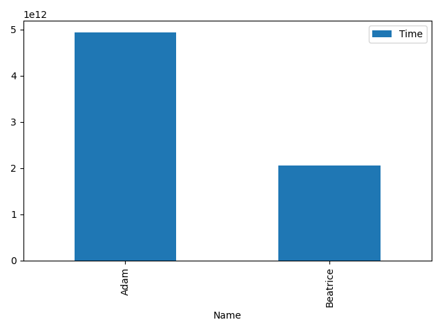
As we see in the bar we have the names, and possibly the times to but the times are written in nano seconds and tends to be quite hard to understand. So lets revise this somewhat and lets use matplotlib instead.
 1: print(df)
 2:
 3: def transform_time(x):
 4:         hours = int(x.components.hours)
 5:         minutes = int(x.components.minutes)
 6:         seconds = int(x.components.seconds)
 7:         microseconds = int(x.microseconds/1000)
 8:         output = f"{hours:02}:{minutes:02}:{seconds:02}.{microseconds:03}"
 9:         print(f"Output: {output}")
10:         return output
11:
12:
13:
14:
15: fig,ax = plt.subplots(figsize=(10, 7))
16: ax.bar(df['Name'], df['Time'].dt.total_seconds()) #
17: ax.set_yticks(df['Time'].dt.total_seconds())
18:
19: plt.yticks(rotation=45)   #
20: plt.tight_layout(pad=3.5) #
21:
22: ax.set_yticklabels(df['Time'].apply( transform_time ) )#
23: #ax.set_yticklabels(df['Name'].str.toupper())
24:
25:
26: # Save the plot to a file
27: output_file = 'py_parse_time_2.png'
28: plt.savefig(output_file)
29: plt.close()
       Name                   Time
0      Adam 0 days 01:22:23.001000
1  Beatrice 0 days 00:34:23.004000
Output: 01:22:23.001
Output: 00:34:23.004
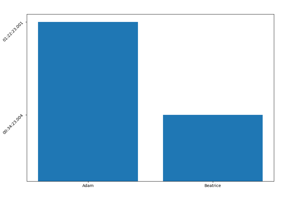
The new revised version has much better resolution, we can actually
see seconds instead of nanoseconds. Line 16 is using the dt
(datetime) accessor to call totalseconds, which is then used in the
y-axis. By setting the set_yticklabels method we can transform the
seconds to a more readable form for each of the y ticks see line
22. Another small adjustment is line 19 which rotates the
y label by 45°, and left pad (line 20) so that the complete text
fits inside the figure, it we skipped the last part there would be a
cut off which only shows about half of the time (e.g 23:004).
Making plots
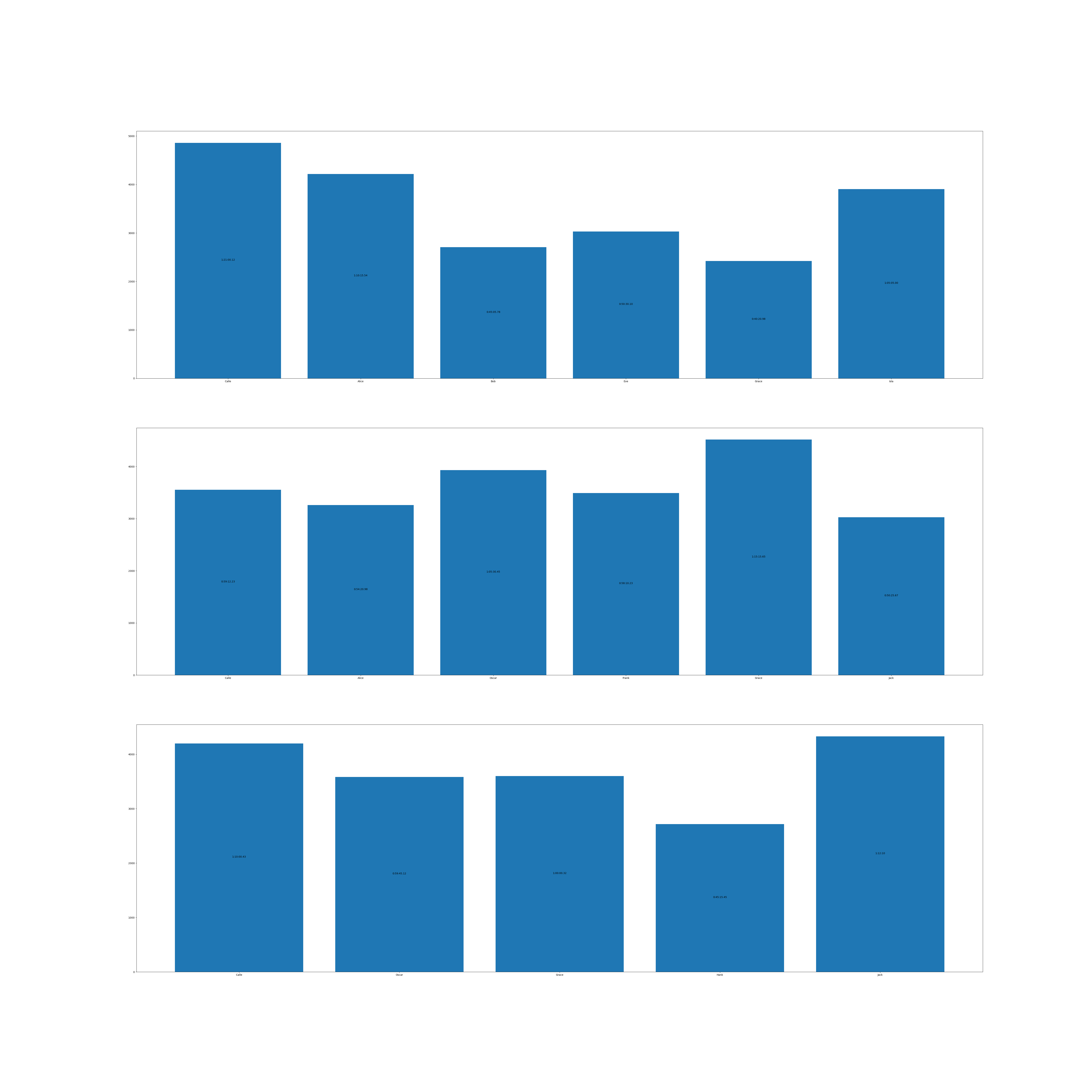
Now we get to the point that we actually want to do some proper plots. We already seen how we can make a bar plot that represent time and some other entity. Since we have our table, we want to make a bar plot for each of the stages. So lets dig into to what needs to be done.
- Import the necessary packages pandas,/matplotlib/
- Create a data frame with all the data from the table
- Convert the times to delta time for easier handling
- create a plots
- The number of plots should match the number of stages, so each plot would make one stage.
- We neeed to figure out how many unique stages we are currently working on
- call matplotlib to create a number of plots
- The number of plots should match the number of stages, so each plot would make one stage.
- For each stage (grouped by stage)
- One axes (figure) , taken from the plot that were created in 3.
- group by stages store the values in appropriate list
- The name (x-axis)
- The value, the position is the same, so no worries. (y-axis)
- Add the x value to the plot
- Save the graphs.
This is the basic idea, there are probably other ways of doing this, but this seems like reasonable especially since that is what we done in the above example.
import pandas as pd
from datetime import datetime,timedelta
from pprint import pprint
from functools import reduce
import matplotlib.pyplot as plt


def transform_time(x):
        hours = int(x.components.hours)
        minutes = int(x.components.minutes)
        seconds = int(x.components.seconds)
        microseconds = int(x.microseconds/1000)
        output = f"{hours:02}:{minutes:02}:{seconds:02}.{microseconds:03}"
        return output

def create_dataframe(data:list[list], columns:list)->pd.DataFrame:
    #Create dataframe
    df = pd.DataFrame(data=data, columns=columns)
    # Make timedelta from the Time field
    df['Time'] = pd.to_timedelta(df['Time'])

    return df

def make_plot(number_stages:int):
    return plt.subplots(number_stages, figsize=(60,60))

def get_unique(data:pd.DataFrame, column: str) -> list:
    return data[column].unique()

def add_labels(x:list ,y:list, axes):
  for i in range(len(x)):
          duration = str(timedelta(seconds=y[i]))
          # To make the %hh:%mm:%ss.ff in the same length
          if len(duration) > 11:
                  diff = len(duration) - 10
                  duration = duration[:-diff]
          axes.text(i, y[i]//2, duration, ha = 'center')


def handle_stages(data_values, stage_group):
    stage, data = stage_group
    all_axes = data_values['axes']
    ax = all_axes[stage-1]
    x_values = data['Name'].values.astype(str)
    y_values = data['Time'].dt.total_seconds()
    ax.bar(x_values,y_values)
    #ax.set_yticks(df['Time'].dt.total_seconds())
    #ax.set_yticklabels(df['Time'].sort_values(ascending=True).apply( transform_time ), ha='right' )
    add_labels(x_values,y_values.values,ax)
    return data_values


df = create_dataframe(data,header)
lst_unique_stages = get_unique(df,'Stage')
fig, axes = make_plot(len(lst_unique_stages))
stage_group = df.groupby('Stage')
reduce(handle_stages, stage_group, {'axes': axes})
#plt.yticks(rotation=45)   # (rot)
#plt.tight_layout(pad=3.5) # (pad)
output_file = 'bar_plot_times.png'
plt.savefig(output_file)
plt.close()

print(f"[[file:bar_plot_times.png]]")

Lets stop there for now, we can of course make this bar much nicer with colors and what else.
But the basic bar is there, a bar graph is nice, but even nicer if we had a plot graph for each riders,
to compare.
Lets think of what we need in that case.
- x axis
- Each of the stages should be represented in the x-axis
- Get the number of unique stages
- y axis
- Each rider should have there own plot.
So for example rider Calle should make its own graph plot with
| x_value | 1 | 2 | 3 |
|---|---|---|---|
| y_value | stage1 time | stage2 time | stage3 time |
If we consider the method we used before, we could instead of grouping with stage we can group with name. This will give us times for each of rider.
 1: import numpy as np
 2: def convert_to_time_repr(seconds: float):
 3:     return str(timedelta(seconds=seconds))
 4:
 5:
 6:
 7: def handle_stage_name(init_values, stage):
 8:     data = init_values['data']
 9:     vals = init_values['times']
10:     stage_value = data[data['Stage'] == stage]['Time']
11:
12:     if len(stage_value) != 0:
13:         val=stage_value.dt.total_seconds().iloc[0]
14:         vals[int(stage)-1] = val
15:     return init_values
16:
17:
18:
19: def handle_name(init_values, name_group):
20:     name,data = name_group
21:     unique_stages = init_values['stages']
22:     ax = init_values['ax']
23:     times = np.full(len(unique_stages), np.nan)
24:
25:     rider_vals = reduce(handle_stage_name,unique_stages, {'data': data, 'times': times} )
26:     ax.plot(unique_stages, rider_vals['times'],'o-', label=name[0])
27:
28:     ax.set_xticks(unique_stages)
29:     ax.set_xlabel('Stages')
30:     init_values[name[0]] = rider_vals['times']
31:
32:     return init_values
33:
34:
35:
36: unique_stages = df['Stage'].unique()
37: name_group = df.groupby(['Name'])
38: fig,ax=plt.subplots( figsize=(16,8))
39: y_values = reduce(handle_name, name_group, {'stages': unique_stages, 'ax': ax })
40: ax.legend()
41: yticks = ax.get_yticks()
42: ax.set_yticks(yticks)  # Set the tick positions first
43: tm_arr = map(convert_to_time_repr, yticks)
44: ax.set_yticklabels(tm_arr, ha='right' )
45:
46: output_file = 'plot_rider_times.png'
47: plt.savefig(output_file)
48: plt.close()
49:
50: print(f"[[file:{output_file}]]")
51:
52:
53:
54:
55:
[[file:plot_rider_times.png]]
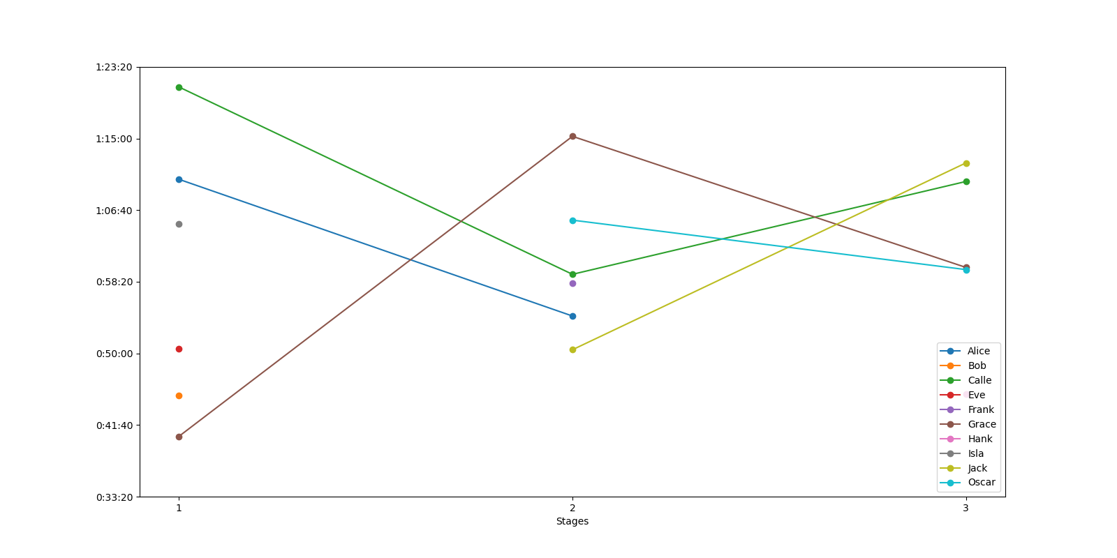
This can obviously be worked on alot more, but the basic idea of how to plot is done.